Chapter 3 The Tidyverse
There is no point in becoming fluent in Enochian if you do not then call forth a Dweller Beneath at the time of the new moon. Similarly, there is no point learning a language designed for data manipulation if you do not then bend data to your will. This chapter therefore looks at how to do the things that R was summoned—er, designed—to do.
3.1 Learning Objectives
- Install and load packages in R.
- Read CSV data with R.
- Explain what a tibble is and how tibbles related to data frames and matrices.
- Describe how
read_csvinfers data types for columns in tabular datasets. - Name and use three functions for inspects tibbles.
- Select subsets of tabular data using column names, scalar indices, ranges, and logical expressions.
- Explain the difference between indexing with
[and with[[. - Name and use four functions for calculating aggregate statistics on tabular data.
- Explain how these functions treat
NAby default, and how to change that behavior.
3.2 How do I read data?
We begin by looking at the file results/infant_hiv.csv,
a tidied version of data on the percentage of infants born to women with HIV
who received an HIV test themselves within two months of birth.
The original data comes from the UNICEF site at https://data.unicef.org/resources/dataset/hiv-aids-statistical-tables/,
and this file contains:
country,year,estimate,hi,lo
AFG,2009,NA,NA,NA
AFG,2010,NA,NA,NA
...
AFG,2017,NA,NA,NA
AGO,2009,NA,NA,NA
AGO,2010,0.03,0.04,0.02
AGO,2011,0.05,0.07,0.04
AGO,2012,0.06,0.08,0.05
...
ZWE,2016,0.71,0.88,0.62
ZWE,2017,0.65,0.81,0.57
The actual file has many more rows (and no ellipses).
It uses NA to show missing data rather than (for example) -, a space, or a blank,
and its values are interpreted as follows:
| Header | Datatype | Description |
|---|---|---|
| country | char | ISO3 country code of country reporting data |
| year | integer | year CE for which data reported |
| estimate | double/NA | estimated percentage of measurement |
| hi | double/NA | high end of range |
| lo | double/NA | low end of range |
We can load this data in Python like this:
     country  year  estimate    hi    lo
0        AFG  2009       NaN   NaN   NaN
1        AFG  2010       NaN   NaN   NaN
2        AFG  2011       NaN   NaN   NaN
3        AFG  2012       NaN   NaN   NaN
4        AFG  2013       NaN   NaN   NaN
...      ...   ...       ...   ...   ...
1723     ZWE  2013      0.57  0.70  0.49
1724     ZWE  2014      0.54  0.67  0.47
1725     ZWE  2015      0.59  0.73  0.51
...
The equivalent in R is to load
the tidyverse collection of packages
and then call the read_csv function.
We will go through this in stages, since each produces output.
Error in library(tidyverse) : there is no package called 'tidyverse'Ah. We must install the tidyverse (but only need to do so once per machine):
At any time,
we can call sessionInfo to find out what versions of which packages we have loaded,
along with the version of R we’re using and some other useful information:
R version 3.6.0 (2019-04-26)
Platform: x86_64-apple-darwin15.6.0 (64-bit)
Running under: macOS High Sierra 10.13.6

Matrix products: default
BLAS:   /Library/Frameworks/R.framework/Versions/3.6/Resources/lib/libRblas.0.dylib
LAPACK: /Library/Frameworks/R.framework/Versions/3.6/Resources/lib/libRlapack.dylib

locale:
[1] en_CA.UTF-8/en_CA.UTF-8/en_CA.UTF-8/C/en_CA.UTF-8/en_CA.UTF-8

attached base packages:
[1] stats     graphics  grDevices utils     datasets  methods   base

other attached packages:
 [1] kableExtra_1.1.0   here_0.1           glue_1.4.1         knitr_1.29
 [5] rlang_0.4.6        reticulate_1.12    forcats_0.4.0      stringr_1.4.0
 [9] dplyr_1.0.0        purrr_0.3.4        readr_1.3.1        tidyr_1.0.0
[13] tibble_3.0.1       ggplot2_3.3.2.9000 tidyverse_1.2.1

loaded via a namespace (and not attached):
 [1] tidyselect_1.1.0  xfun_0.15         haven_2.1.1       lattice_0.20-38
 [5] colorspace_1.4-1  vctrs_0.3.1       generics_0.0.2    htmltools_0.5.0
 [9] viridisLite_0.3.0 yaml_2.2.1        pillar_1.4.4      withr_2.2.0
[13] modelr_0.1.5      readxl_1.3.1      lifecycle_0.2.0   munsell_0.5.0
[17] gtable_0.3.0      cellranger_1.1.0  rvest_0.3.6       evaluate_0.14
[21] fansi_0.4.1       broom_0.5.2       Rcpp_1.0.4.6      scales_1.1.1
[25] backports_1.1.8   webshot_0.5.1     jsonlite_1.7.0    hms_0.5.0
[29] digest_0.6.25     stringi_1.4.6     bookdown_0.19     grid_3.6.0
[33] rprojroot_1.3-2   cli_2.0.2         tools_3.6.0       magrittr_1.5
[37] crayon_1.3.4      pkgconfig_2.0.3   ellipsis_0.3.1    Matrix_1.2-17
[41] xml2_1.3.2        lubridate_1.7.9   assertthat_0.2.1  rmarkdown_2.2
[45] httr_1.4.1        rstudioapi_0.11   R6_2.4.1          nlme_3.1-140
[49] compiler_3.6.0
We then load the library once per program:
Note that we give install.packages a string to install,
but simply give the name of the package we want to load to library.
Loading the tidyverse gives us eight packages.
One of those, dplyr, defines two functions that mask standard functions in R with the same names.
If we need the originals,
we can always get them with their
fully-qualified names
stats::filter and stats::lag.
Once we have the tidyverse loaded, reading the file looks remarkably like reading the file:
Parsed with column specification:
cols(
  country = col_character(),
  year = col_double(),
  estimate = col_double(),
  hi = col_double(),
  lo = col_double()
)
R’s read_csv tells us more about what it has done than Pandas does.
In particular, it guesses the data types of columns based on the first thousand values
and then tells us what types it has inferred.
(In a better universe,
people would habitually use the first two rows of their spreadsheets for name and units,
but we do not live there.)
We can now look at what read_csv has produced.
# A tibble: 1,728 x 5
   country  year estimate    hi    lo
   <chr>   <dbl>    <dbl> <dbl> <dbl>
 1 AFG      2009       NA    NA    NA
 2 AFG      2010       NA    NA    NA
 3 AFG      2011       NA    NA    NA
 4 AFG      2012       NA    NA    NA
 5 AFG      2013       NA    NA    NA
 6 AFG      2014       NA    NA    NA
 7 AFG      2015       NA    NA    NA
 8 AFG      2016       NA    NA    NA
 9 AFG      2017       NA    NA    NA
10 AGO      2009       NA    NA    NA
# … with 1,718 more rows
This is a tibble,
which is the tidyverse’s enhanced version of R’s data.frame.
It organizes data into named columns,
each having one value for each row.
In statistical terms,
the columns are the variables being observed
and the rows are the actual observations.
3.3 How do I inspect data?
We often have a quick look at the content of a table to remind ourselves what it contains.
Pandas does this using methods whose names are borrowed from the Unix shell’s head and tail commands:
  country  year  estimate  hi  lo
0     AFG  2009       NaN NaN NaN
1     AFG  2010       NaN NaN NaN
2     AFG  2011       NaN NaN NaN
3     AFG  2012       NaN NaN NaN
4 AFG 2013 NaN NaN NaN country year estimate hi lo
1723 ZWE 2013 0.57 0.70 0.49
1724 ZWE 2014 0.54 0.67 0.47
1725 ZWE 2015 0.59 0.73 0.51
1726 ZWE 2016 0.71 0.88 0.62
1727 ZWE 2017 0.65 0.81 0.57R has similarly-named functions:
# A tibble: 6 x 5
  country  year estimate    hi    lo
  <chr>   <dbl>    <dbl> <dbl> <dbl>
1 AFG      2009       NA    NA    NA
2 AFG      2010       NA    NA    NA
3 AFG      2011       NA    NA    NA
4 AFG      2012       NA    NA    NA
5 AFG      2013       NA    NA    NA
6 AFG 2014 NA NA NA# A tibble: 6 x 5
country year estimate hi lo
<chr> <dbl> <dbl> <dbl> <dbl>
1 ZWE 2012 0.38 0.47 0.33
2 ZWE 2013 0.570 0.7 0.49
3 ZWE 2014 0.54 0.67 0.47
4 ZWE 2015 0.59 0.73 0.51
5 ZWE 2016 0.71 0.88 0.62
6 ZWE 2017 0.65 0.81 0.570Let’s have a closer look at that last command’s output:
# A tibble: 6 x 5
  country  year estimate    hi    lo
  <chr>   <dbl>    <dbl> <dbl> <dbl>
1 ZWE      2012    0.38   0.47 0.33
2 ZWE      2013    0.570  0.7  0.49
3 ZWE      2014    0.54   0.67 0.47
4 ZWE      2015    0.59   0.73 0.51
5 ZWE      2016    0.71   0.88 0.62
6 ZWE 2017 0.65 0.81 0.570Note that the row numbers printed by tail are relative to the output,
not absolute to the table.
This is different from Pandas,
which retains the original row numbers.
What about overall information?
<class 'pandas.core.frame.DataFrame'>
RangeIndex: 1728 entries, 0 to 1727
Data columns (total 5 columns):
country     1728 non-null object
year        1728 non-null int64
estimate    728 non-null float64
hi          728 non-null float64
lo          728 non-null float64
dtypes: float64(3), int64(1), object(1)
memory usage: 67.6+ KB
None country year estimate hi
Length:1728 Min. :2009 Min. :0.000 Min. :0.0000
Class :character 1st Qu.:2011 1st Qu.:0.100 1st Qu.:0.1400
Mode :character Median :2013 Median :0.340 Median :0.4350
Mean :2013 Mean :0.387 Mean :0.4614
3rd Qu.:2015 3rd Qu.:0.620 3rd Qu.:0.7625
Max. :2017 Max. :0.950 Max. :0.9500
NA's :1000 NA's :1000
lo
Min. :0.0000
1st Qu.:0.0800
Median :0.2600
Mean :0.3221
3rd Qu.:0.5100
Max. :0.9500
NA's :1000 Your display of R’s summary may or may not wrap, depending on how large a screen the older acolytes have allowed you.
3.4 How do I index rows and columns?
A Pandas DataFrame is a collection of series (also called columns), each containing the values of a single observed variable:
0        NaN
1        NaN
2        NaN
3        NaN
4        NaN
        ...
1723    0.57
1724    0.54
1725    0.59
1726    0.71
1727    0.65
Name: estimate, Length: 1728, dtype: float64
We would get exactly the same output in Python with infant_hiv.estimate,
i.e.,
with an attribute name rather than a string subscript.
The same tricks work in R:
# A tibble: 1,728 x 1
   estimate
      <dbl>
 1       NA
 2       NA
 3       NA
 4       NA
 5       NA
 6       NA
 7       NA
 8       NA
 9       NA
10       NA
# … with 1,718 more rows
However, R’s infant_hiv$estimate provides all the data:
   [1]   NA   NA   NA   NA   NA   NA   NA   NA   NA   NA 0.03 0.05 0.06 0.15
  [15] 0.10 0.06 0.01 0.01   NA   NA   NA   NA   NA   NA   NA   NA   NA   NA
  [29]   NA   NA   NA   NA   NA   NA   NA   NA   NA   NA   NA   NA   NA   NA
  [43]   NA   NA   NA   NA   NA 0.13 0.12 0.12 0.52 0.53 0.67 0.66   NA   NA
  [57]   NA   NA   NA   NA   NA   NA   NA   NA   NA   NA   NA   NA   NA   NA
  [71]   NA   NA   NA   NA   NA   NA   NA   NA   NA   NA   NA   NA   NA   NA
  [85]   NA   NA   NA   NA   NA   NA 0.26 0.24 0.38 0.55 0.61 0.74 0.83 0.75
  [99] 0.74   NA 0.10 0.10 0.11 0.18 0.12 0.02 0.12 0.20   NA   NA   NA   NA
 [113]   NA   NA   NA   NA   NA   NA   NA 0.10 0.09 0.12 0.26 0.27 0.25 0.32
 [127] 0.03 0.09 0.13 0.19 0.25 0.30 0.28 0.15 0.16   NA 0.02 0.02 0.02 0.03
 [141] 0.15 0.10 0.17 0.14   NA   NA   NA   NA   NA   NA   NA   NA   NA   NA
 [155]   NA   NA   NA   NA   NA   NA   NA   NA   NA   NA   NA   NA   NA   NA
 [169]   NA   NA   NA   NA   NA   NA   NA   NA   NA   NA   NA   NA 0.95 0.95
 [183] 0.95 0.95 0.95 0.95 0.80 0.95 0.87 0.77 0.75 0.72 0.51 0.55 0.50 0.62
 [197] 0.37 0.36 0.07 0.46 0.46 0.46 0.46 0.44 0.43 0.42 0.40 0.25 0.25 0.46
 [211] 0.25 0.45 0.45 0.46 0.46 0.45   NA   NA   NA   NA   NA   NA   NA   NA
 [225]   NA   NA   NA   NA   NA   NA   NA   NA   NA   NA   NA   NA   NA   NA
 [239]   NA   NA   NA   NA   NA   NA 0.53 0.35 0.36 0.48 0.41 0.45 0.47 0.50
 [253] 0.01 0.01 0.07 0.05 0.03 0.09 0.12 0.21 0.23   NA   NA   NA   NA   NA
 [267]   NA   NA   NA   NA   NA   NA   NA   NA   NA   NA   NA   NA   NA   NA
...
Again, note that the boxed number on the left is the start index of that row.
What about single values? Remembering to count from zero from Python and as humans do for R, we have:
0.05[1] 0.05Ah—everything in R is a vector, so we get a vector of one value as an output rather than a single value.
Error in py_call_impl(callable, dots$args, dots$keywords): TypeError: object of type 'numpy.float64' has no len()

Detailed traceback:
File "<string>", line 1, in <module>[1] 1And yes, ranges work:
5      NaN
6      NaN
7      NaN
8      NaN
9      NaN
10    0.03
11    0.05
12    0.06
13    0.15
14    0.10
Name: estimate, dtype: float64 [1] NA NA NA NA NA 0.03 0.05 0.06 0.15 0.10Note that the upper bound is the same, because it’s inclusive in R and exclusive in Python. Note also that nothing prevents us from selecting a range of rows that spans several countries, which is why selecting by row number is usually a sign of innocence, insouciance, or desperation.
We can select by column number as well.
Pandas uses the rather clumsy object.iloc[rows, columns] with the usual shortcut : for “entire range”:
0       AFG
1       AFG
2       AFG
3       AFG
4       AFG
       ...
1723    ZWE
1724    ZWE
1725    ZWE
1726    ZWE
1727    ZWE
Name: country, Length: 1728, dtype: object
Since this is a column, it can be indexed:
AFGIn R, a single index is interpreted as the column index:
# A tibble: 1,728 x 1
   country
   <chr>
 1 AFG
 2 AFG
 3 AFG
 4 AFG
 5 AFG
 6 AFG
 7 AFG
 8 AFG
 9 AFG
10 AGO
# … with 1,718 more rows
But notice that the output is not a vector, but another tibble (i.e., a table with N rows and one column). This means that adding another index does column-wise indexing on that tibble:
# A tibble: 1,728 x 1
   country
   <chr>
 1 AFG
 2 AFG
 3 AFG
 4 AFG
 5 AFG
 6 AFG
 7 AFG
 8 AFG
 9 AFG
10 AGO
# … with 1,718 more rows
How then are we to get the first mention of Afghanistan? The answer is to use double square brackets to strip away one level of structure:
   [1] "AFG" "AFG" "AFG" "AFG" "AFG" "AFG" "AFG" "AFG" "AFG" "AGO" "AGO" "AGO"
  [13] "AGO" "AGO" "AGO" "AGO" "AGO" "AGO" "AIA" "AIA" "AIA" "AIA" "AIA" "AIA"
  [25] "AIA" "AIA" "AIA" "ALB" "ALB" "ALB" "ALB" "ALB" "ALB" "ALB" "ALB" "ALB"
  [37] "ARE" "ARE" "ARE" "ARE" "ARE" "ARE" "ARE" "ARE" "ARE" "ARG" "ARG" "ARG"
  [49] "ARG" "ARG" "ARG" "ARG" "ARG" "ARG" "ARM" "ARM" "ARM" "ARM" "ARM" "ARM"
  [61] "ARM" "ARM" "ARM" "ATG" "ATG" "ATG" "ATG" "ATG" "ATG" "ATG" "ATG" "ATG"
  [73] "AUS" "AUS" "AUS" "AUS" "AUS" "AUS" "AUS" "AUS" "AUS" "AUT" "AUT" "AUT"
  [85] "AUT" "AUT" "AUT" "AUT" "AUT" "AUT" "AZE" "AZE" "AZE" "AZE" "AZE" "AZE"
  [97] "AZE" "AZE" "AZE" "BDI" "BDI" "BDI" "BDI" "BDI" "BDI" "BDI" "BDI" "BDI"
 [109] "BEL" "BEL" "BEL" "BEL" "BEL" "BEL" "BEL" "BEL" "BEL" "BEN" "BEN" "BEN"
 [121] "BEN" "BEN" "BEN" "BEN" "BEN" "BEN" "BFA" "BFA" "BFA" "BFA" "BFA" "BFA"
 [133] "BFA" "BFA" "BFA" "BGD" "BGD" "BGD" "BGD" "BGD" "BGD" "BGD" "BGD" "BGD"
 [145] "BGR" "BGR" "BGR" "BGR" "BGR" "BGR" "BGR" "BGR" "BGR" "BHR" "BHR" "BHR"
 [157] "BHR" "BHR" "BHR" "BHR" "BHR" "BHR" "BHS" "BHS" "BHS" "BHS" "BHS" "BHS"
 [169] "BHS" "BHS" "BHS" "BIH" "BIH" "BIH" "BIH" "BIH" "BIH" "BIH" "BIH" "BIH"
 [181] "BLR" "BLR" "BLR" "BLR" "BLR" "BLR" "BLR" "BLR" "BLR" "BLZ" "BLZ" "BLZ"
 [193] "BLZ" "BLZ" "BLZ" "BLZ" "BLZ" "BLZ" "BOL" "BOL" "BOL" "BOL" "BOL" "BOL"
 [205] "BOL" "BOL" "BOL" "BRA" "BRA" "BRA" "BRA" "BRA" "BRA" "BRA" "BRA" "BRA"
 [217] "BRB" "BRB" "BRB" "BRB" "BRB" "BRB" "BRB" "BRB" "BRB" "BRN" "BRN" "BRN"
 [229] "BRN" "BRN" "BRN" "BRN" "BRN" "BRN" "BTN" "BTN" "BTN" "BTN" "BTN" "BTN"
...
This is now a plain old vector, so it can be indexed with single square brackets:
[1] "AFG"But that too is a vector, so it can of course be indexed as well (for some value of “of course”):
[1] "AFG"Thus,
data[1][[1]] produces a tibble,
then selects the first column vector from it,
so it still gives us a vector.
This is not madness.
It is merely…differently sane.
Subsetting Data Frames
When we are working with data frames (including tibbles), subsetting with a single vector selects columns, not rows, because data frames are stored as lists of columns. This means that
df[1:2]selects two columns fromdf. However, indf[2:3, 1:2], the first index selects rows, while the second selects columns.
3.5 How do I calculate basic statistics?
What is the average estimate? We start by grabbing that column for convenience:
17280.3870192307692308This translates almost directly to R:
[1] 1728[1] NAThe void is always there, waiting for us…
Let’s fix this in R first by telling mean to drop NAs:
[1] 0.3870192and then try to get the statistically correct behavior in Pandas:
nanMany functions in R use na.rm to control whether NAs are removed or not.
(Remember, the . character is just another part of the name)
R’s default behavior is to leave NAs in, and then to include them in aggregate computations.
Python’s is to get rid of missing values early and work with what’s left,
which makes translating code from one language to the next much more interesting than it might otherwise be.
But other than that, the statistics works the same way.
In Python, we write:
min 0.0max 0.95std 0.3034511074214113and in R:
min 0max 0.95sd 0.303451107421411A good use of aggregation is to check the quality of the data. For example, we can ask if there are any records where some of the estimate, the low value, or the high value are missing, but not all of them:
False[1] FALSE3.6 How do I filter data?
By “filtering”, we mean “selecting records by value”.
As discussed in Chapter 2,
the simplest approach is to use a vector of logical values to keep only the values corresponding to TRUE.
In Python, this is:
52And in R:
[1] 1052The difference is unexpected. Let’s have a closer look at the result in Python:
180     0.95
181     0.95
182     0.95
183     0.95
184     0.95
185     0.95
187     0.95
360     0.95
361     0.95
362     0.95
379     0.95
380     0.95
381     0.95
382     0.95
384     0.95
385     0.95
386     0.95
446     0.95
447     0.95
461     0.95
...
And in R:
   [1]   NA   NA   NA   NA   NA   NA   NA   NA   NA   NA   NA   NA   NA   NA
  [15]   NA   NA   NA   NA   NA   NA   NA   NA   NA   NA   NA   NA   NA   NA
  [29]   NA   NA   NA   NA   NA   NA   NA   NA   NA   NA   NA   NA   NA   NA
  [43]   NA   NA   NA   NA   NA   NA   NA   NA   NA   NA   NA   NA   NA   NA
  [57]   NA   NA   NA   NA   NA   NA   NA   NA   NA   NA   NA   NA   NA   NA
  [71]   NA   NA   NA   NA   NA   NA   NA   NA   NA   NA   NA   NA   NA   NA
  [85]   NA   NA   NA   NA   NA   NA   NA   NA   NA   NA   NA   NA   NA   NA
  [99]   NA   NA   NA   NA   NA   NA   NA   NA   NA   NA   NA   NA   NA   NA
 [113]   NA   NA   NA   NA   NA   NA   NA   NA   NA   NA   NA   NA 0.95 0.95
 [127] 0.95 0.95 0.95 0.95 0.95   NA   NA   NA   NA   NA   NA   NA   NA   NA
 [141]   NA   NA   NA   NA   NA   NA   NA   NA   NA   NA   NA   NA   NA   NA
 [155]   NA   NA   NA   NA   NA   NA   NA   NA   NA   NA   NA   NA   NA   NA
 [169]   NA   NA   NA   NA   NA   NA   NA   NA   NA   NA   NA   NA   NA   NA
 [183]   NA   NA   NA   NA   NA   NA   NA   NA   NA   NA   NA   NA   NA   NA
 [197]   NA   NA   NA   NA   NA   NA   NA   NA   NA   NA   NA   NA 0.95 0.95
 [211] 0.95 0.95 0.95 0.95 0.95 0.95 0.95 0.95   NA   NA   NA   NA   NA   NA
 [225]   NA   NA   NA   NA   NA   NA   NA   NA   NA   NA   NA   NA   NA   NA
 [239]   NA   NA   NA   NA   NA   NA   NA   NA   NA   NA   NA   NA   NA   NA
 [253]   NA   NA   NA   NA   NA   NA   NA   NA   NA   NA   NA   NA   NA 0.95
 [267] 0.95   NA   NA 0.95   NA   NA   NA   NA   NA   NA   NA   NA   NA   NA
...
It appears that R has kept the unknown values in order to highlight just how little we know.
More precisely,
wherever there was an NA in the original data
there is an NA in the logical vector
and hence an NA in the final vector.
Let us then turn to which to get a vector of indices at which a vector contains TRUE.
This function does not return indices for FALSE or NA:
 [1]  181  182  183  184  185  186  188  361  362  363  380  381  382  383  385
[16]  386  387  447  448  462  793  794  795  796  797  798  911  912  955  956
[31]  957  958  959  960  961  962  963 1098 1107 1128 1429 1430 1462 1554 1604
[46] 1607 1625 1626 1627 1629 1708 1710
And as a quick check:
[1] 52So now we can index our vector with the result of the which:
 [1] 0.95 0.95 0.95 0.95 0.95 0.95 0.95 0.95 0.95 0.95 0.95 0.95 0.95 0.95 0.95
[16] 0.95 0.95 0.95 0.95 0.95 0.95 0.95 0.95 0.95 0.95 0.95 0.95 0.95 0.95 0.95
[31] 0.95 0.95 0.95 0.95 0.95 0.95 0.95 0.95 0.95 0.95 0.95 0.95 0.95 0.95 0.95
[46] 0.95 0.95 0.95 0.95 0.95 0.95 0.95
But should we do this?
Those NAs are important information,
and should not be discarded so blithely.
What we should really be doing is using the tools the tidyverse provides
rather than clever indexing tricks.
These behave consistently across a wide scale of problems
and encourage use of patterns that make it easier for others to understand our programs.
3.7 How do I write tidy code?
The six basic data transformation operations in the tidyverse are:
filter: choose observations (rows) by value(s)arrange: reorder rowsselect: choose variables (columns) by namemutate: derive new variables from existing onesgroup_by: define subsets of rows for further processingsummarize: combine many values to create a single new value
filter(tibble, ...criteria...) keeps rows that pass all of the specified criteria:
# A tibble: 183 x 5
   country  year estimate    hi    lo
   <chr>   <dbl>    <dbl> <dbl> <dbl>
 1 ARG      2016     0.67  0.77  0.61
 2 ARG      2017     0.66  0.77  0.6
 3 AZE      2014     0.74  0.95  0.53
 4 AZE      2015     0.83  0.95  0.64
 5 AZE      2016     0.75  0.95  0.56
 6 AZE      2017     0.74  0.95  0.56
 7 BLR      2009     0.95  0.95  0.95
 8 BLR      2010     0.95  0.95  0.95
 9 BLR      2011     0.95  0.95  0.91
10 BLR      2012     0.95  0.95  0.95
# … with 173 more rows
Notice that the expression is lo > 0.5 rather than "lo" > 0.5.
The latter expression would return the entire table
because the string "lo" is greater than the number 0.5 everywhere.
But how is it that the name lo can be used on its own?
It is the name of a column, but there is no variable called lo.
The answer is that R uses lazy evaluation:
function arguments aren’t evaluated until they’re needed,
so the function filter actually gets the expression lo > 0.5,
which allows it to check that there’s a column called lo and then use it appropriately.
It may seem strange at first,
but it is much tidier than filter(data, data$lo > 0.5) or filter(data, "lo > 0.5").
We will explore lazy evaluation further in Chapter 6.
We can make data anlaysis code more readable by using the pipe operator %>%:
# A tibble: 183 x 5
   country  year estimate    hi    lo
   <chr>   <dbl>    <dbl> <dbl> <dbl>
 1 ARG      2016     0.67  0.77  0.61
 2 ARG      2017     0.66  0.77  0.6
 3 AZE      2014     0.74  0.95  0.53
 4 AZE      2015     0.83  0.95  0.64
 5 AZE      2016     0.75  0.95  0.56
 6 AZE      2017     0.74  0.95  0.56
 7 BLR      2009     0.95  0.95  0.95
 8 BLR      2010     0.95  0.95  0.95
 9 BLR      2011     0.95  0.95  0.91
10 BLR      2012     0.95  0.95  0.95
# … with 173 more rows
This may not seem like much of an improvement,
but neither does a Unix pipe consisting of cat filename.txt | head.
What about this?
# A tibble: 1 x 5
  country  year estimate    hi    lo
  <chr>   <dbl>    <dbl> <dbl> <dbl>
1 TTO      2017     0.94  0.95  0.86
It uses the vectorized “and” operator & twice,
and parsing the condition takes a human being at least a few seconds.
Its pipelined equivalent is:
# A tibble: 1 x 5
  country  year estimate    hi    lo
  <chr>   <dbl>    <dbl> <dbl> <dbl>
1 TTO      2017     0.94  0.95  0.86
Breaking the condition into stages like this often makes reading and testing much easier,
and encourages incremental write-test-extend development.
Let’s increase the band from 10% to 20%,
break the line the way the tidyverse style guide recommends
to make the operations easier to spot,
and order by lo in descending order:
infant_hiv %>%
  filter(estimate != 0.95) %>%
  filter(lo > 0.5) %>%
  filter(hi <= (lo + 0.2)) %>%
  arrange(desc(lo))
# A tibble: 55 x 5
country year estimate hi lo
<chr> <dbl> <dbl> <dbl> <dbl>
1 TTO 2017 0.94 0.95 0.86
2 SWZ 2011 0.93 0.95 0.84
3 CUB 2014 0.92 0.95 0.83
4 TTO 2016 0.9 0.95 0.83
5 CRI 2009 0.92 0.95 0.81
6 CRI 2012 0.89 0.95 0.81
7 NAM 2014 0.91 0.95 0.81
8 URY 2016 0.9 0.95 0.81
9 ZMB 2014 0.91 0.95 0.81
10 KAZ 2015 0.84 0.95 0.8
# … with 45 more rowsWe can now select the three columns we care about:
infant_hiv %>%
  filter(estimate != 0.95) %>%
  filter(lo > 0.5) %>%
  filter(hi <= (lo + 0.2)) %>%
  arrange(desc(lo)) %>%
  select(year, lo, hi)
# A tibble: 55 x 3
year lo hi
<dbl> <dbl> <dbl>
1 2017 0.86 0.95
2 2011 0.84 0.95
3 2014 0.83 0.95
4 2016 0.83 0.95
5 2009 0.81 0.95
6 2012 0.81 0.95
7 2014 0.81 0.95
8 2016 0.81 0.95
9 2014 0.81 0.95
10 2015 0.8 0.95
# … with 45 more rowsOnce again,
we are using the unquoted column names year, lo, and hi
and letting R’s lazy evaluation take care of the details for us.
Rather than selecting these three columns,
we can select out the columns we’re not interested in
by negating their names.
This leaves the columns that are kept in their original order,
rather than putting lo before hi,
which won’t matter if we later select by name,
but will if we ever want to select by position:
infant_hiv %>%
  filter(estimate != 0.95) %>%
  filter(lo > 0.5) %>%
  filter(hi <= (lo + 0.2)) %>%
  arrange(desc(lo)) %>%
  select(-country, -estimate)
# A tibble: 55 x 3
year hi lo
<dbl> <dbl> <dbl>
1 2017 0.95 0.86
2 2011 0.95 0.84
3 2014 0.95 0.83
4 2016 0.95 0.83
5 2009 0.95 0.81
6 2012 0.95 0.81
7 2014 0.95 0.81
8 2016 0.95 0.81
9 2014 0.95 0.81
10 2015 0.95 0.8
# … with 45 more rowsGiddy with power,
we now add a column containing the difference between the low and high values.
This can be done using either mutate,
which adds new columns to the end of an existing tibble,
or with transmute,
which creates a new tibble containing only the columns we explicitly ask for.
(There is also a function rename which simply renames columns.)
Since we want to keep hi and lo,
we decide to use mutate:
infant_hiv %>%
  filter(estimate != 0.95) %>%
  filter(lo > 0.5) %>%
  filter(hi <= (lo + 0.2)) %>%
  arrange(desc(lo)) %>%
  select(-country, -estimate) %>%
  mutate(difference = hi - lo)
# A tibble: 55 x 4
year hi lo difference
<dbl> <dbl> <dbl> <dbl>
1 2017 0.95 0.86 0.0900
2 2011 0.95 0.84 0.110
3 2014 0.95 0.83 0.12
4 2016 0.95 0.83 0.12
5 2009 0.95 0.81 0.140
6 2012 0.95 0.81 0.140
7 2014 0.95 0.81 0.140
8 2016 0.95 0.81 0.140
9 2014 0.95 0.81 0.140
10 2015 0.95 0.8 0.150
# … with 45 more rowsDoes the difference between high and low estimates vary by year?
To answer that question,
we use group_by to group records by value
and then summarize to aggregate within groups.
We might as well get rid of the arrange and select calls in our pipeline at this point,
since we’re not using them,
and count how many records contributed to each aggregation using n():
infant_hiv %>%
  filter(estimate != 0.95) %>%
  filter(lo > 0.5) %>%
  filter(hi <= (lo + 0.2)) %>%
  mutate(difference = hi - lo) %>%
  group_by(year) %>%
  summarize(count = n(), ave_diff = mean(year))
`summarise()` ungrouping output (override with `.groups` argument)# A tibble: 9 x 3
year count ave_diff
<dbl> <int> <dbl>
1 2009 3 2009
2 2010 3 2010
3 2011 5 2011
4 2012 5 2012
5 2013 6 2013
6 2014 10 2014
7 2015 6 2015
8 2016 10 2016
9 2017 7 2017How might we do this with Pandas?
One approach is to use a single multi-part .query to select data
and store the result in a variable so that we can refer to the hi and lo columns twice
without repeating the filtering expression.
We then group by year and aggregate, again using strings for column names:
data = pd.read_csv('results/infant_hiv.csv')
data = data.query('(estimate != 0.95) & (lo > 0.5) & (hi <= (lo + 0.2))')
data = data.assign(difference = (data.hi - data.lo))
grouped = data.groupby('year').agg({'difference' : {'ave_diff' : 'mean', 'count' : 'count'}})
//anaconda3/lib/python3.7/site-packages/pandas/core/groupby/generic.py:1455: FutureWarning: using a dict with renaming is deprecated and will be removed
in a future version.
For column-specific groupby renaming, use named aggregation
>>> df.groupby(...).agg(name=('column', aggfunc))
return super().aggregate(arg, *args, **kwargs) difference
ave_diff count
year
2009 0.170000 3
2010 0.186667 3
2011 0.168000 5
2012 0.186000 5
2013 0.183333 6
2014 0.168000 10
2015 0.161667 6
2016 0.166000 10
2017 0.152857 7There are other ways to tackle this problem with Pandas, but the tidyverse approach produces code that I find more readable.
3.8 How do I model my data?
Tidying up data can be as calming and rewarding in the same way as knitting
or rearranging the specimen jars on the shelves in your dining room-stroke-laboratory.
Eventually,
though,
people want to do some statistics.
The simplest tool for this in R is lm, which stands for “linear model”.
Given a formula and a data set,
it calculates coefficients to fit that formula to that data:
Call:
lm(formula = estimate ~ lo, data = infant_hiv)

Coefficients:
(Intercept)           lo
     0.0421       1.0707
This is telling us that estimate is more-or-less equal to 0.0421 + 1.0707 * lo.
The ~ symbol is used to separate the left and right sides of the equation,
and as with all things tidyverse,
lazy evaluation allows us to use variable names directly.
In fact,
it lets us write much more complex formulas involving functions of multiple variables.
For example,
we can regress estimate against the square roots of lo and hi
(though there is no sound statistical reason to do so):
Call:
lm(formula = estimate ~ sqrt(lo) + sqrt(hi), data = infant_hiv)

Coefficients:
(Intercept)     sqrt(lo)     sqrt(hi)
    -0.2225       0.6177       0.4814
One important thing to note here is the way that + is overloaded in formulas.
The formula estimate ~ lo + hi does not mean “regress estimate against the sum of lo and hi”,
but rather, “regress estimate against the two variables lo and hi”:
Call:
lm(formula = estimate ~ lo + hi, data = infant_hiv)

Coefficients:
(Intercept)           lo           hi
   -0.01327      0.42979      0.56752
If we want to regress estimate against the average of lo and hi
(i.e., regress estimate against a single calculated variable instead of against two variables)
we need to create a temporary column:
Call:
lm(formula = estimate ~ ave_lo_hi, data = .)

Coefficients:
(Intercept)    ave_lo_hi
   -0.00897      1.01080
Here, the call to lm is using the variable . to mean
“the data coming in from the previous stage of the pipeline”.
Most of the functions in the tidyverse use this convention
so that data can be passed to a function that expects it in a position other than the first.
3.9 How do I create a plot?
Human being always want to see the previously unseen,
though they are not always glad to have done so.
The most popular tool for doing this in R is ggplot2,
which implements and extends the patterns for creating charts described in Wilkinson (2005).
Every chart it creates has a geometry that controls how data is displayed
and a mapping that controls how values are represented geometrically.
For example,
these lines of code create a scatter plot
showing the relationship between lo and hi values in the infant HIV data:
Warning: Removed 1000 rows containing missing values (geom_point).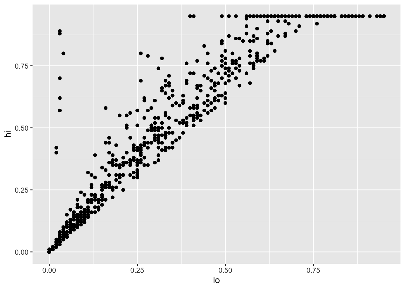
Looking more closely:
- The function
ggplotcreates an object to represent the chart withinfant_hivas the underlying data. geom_pointspecifies the geometry we want (points).- Its
mappingargument is assigned an aesthetic that specifieslois to be used as thexcoordinate andhiis to be used as theycoordinate. - The elements of the chart are combined with
+rather than%>%for historical reasons.
Let’s create a slightly more appealing plot by dropping NAs,
making the points semi-transparent,
and colorizing them according to the value of estimate:
infant_hiv %>%
  drop_na() %>%
  ggplot(mapping = aes(x = lo, y = hi, color = estimate)) +
  geom_point(alpha = 0.5) +
  xlim(0.0, 1.0) + ylim(0.0, 1.0)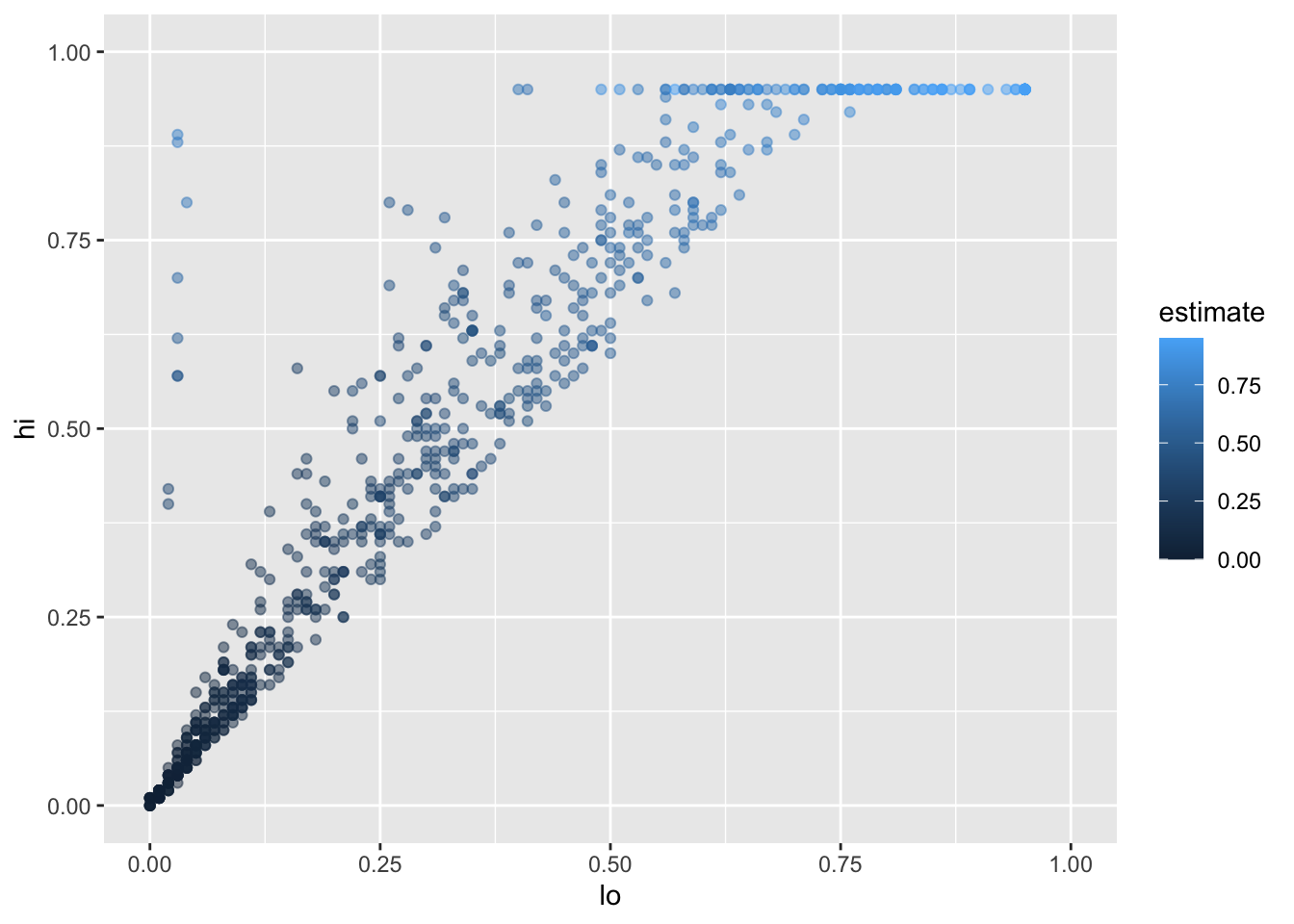
We set the transparency alpha outside the aesthetic because its value is constant for all points.
If we set it inside aes(...),
we would be telling ggplot2 to set the transparency according to the value of the data.
We specify the limits to the axes manually with xlim and ylim to ensure that ggplot2 includes the upper bounds:
without this,
all of the data would be shown,
but the upper label “1.00” would be omitted.
This plot immediately shows us that we have some outliers.
There are far more values with hi equal to 0.95 than it seems there ought to be,
and there are eight points running up the left margin that seem troubling as well.
Let’s create a new tibble that doesn’t have these:
infant_hiv %>%
  drop_na() %>%
  filter(hi != 0.95) %>%
  filter(!((lo < 0.10) & (hi > 0.25))) %>%
  ggplot(mapping = aes(x = lo, y = hi, color = estimate)) +
  geom_point(alpha = 0.5) +
  xlim(0.0, 1.0) + ylim(0.0, 1.0)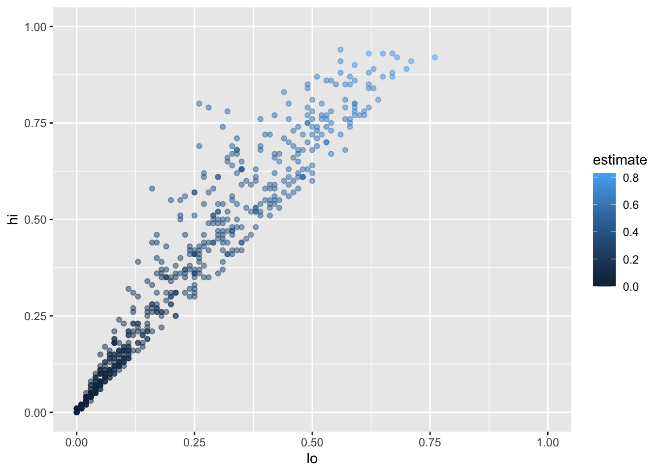
We can add the fitted curve by including another geometry called geom_smooth:
infant_hiv %>%
  drop_na() %>%
  filter(hi != 0.95) %>%
  filter(!((lo < 0.10) & (hi > 0.25))) %>%
  ggplot(mapping = aes(x = lo, y = hi)) +
  geom_point(mapping = aes(color = estimate), alpha = 0.5) +
  geom_smooth(method = lm, color = 'red') +
  xlim(0.0, 1.0) + ylim(0.0, 1.0)
`geom_smooth()` using formula 'y ~ x'Warning: Removed 8 rows containing missing values (geom_smooth).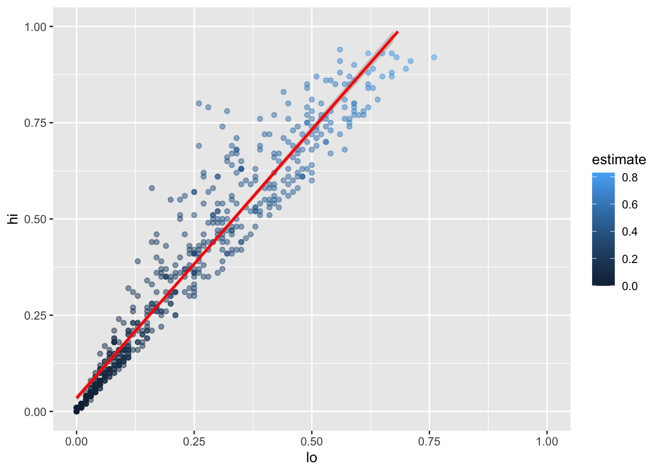
But wait:
why is this complaining about missing values?
Some online searches lead to the discovery that
geom_smooth adds virtual points to the data for plotting purposes,
some of which lie outside the range of the actual data,
and that setting xlim and ylim then truncates these.
(Remember, R is differently sane…)
The safe way to control the range of the data is to add a call to coord_cartesian,
which effectively zooms in on a region of interest:
infant_hiv %>%
  drop_na() %>%
  filter(hi != 0.95) %>%
  filter(!((lo < 0.10) & (hi > 0.25))) %>%
  ggplot(mapping = aes(x = lo, y = hi)) +
  geom_point(mapping = aes(color = estimate), alpha = 0.5) +
  geom_smooth(method = lm, color = 'red') +
  coord_cartesian(xlim = c(0.0, 1.0), ylim = c(0.0, 1.0))
`geom_smooth()` using formula 'y ~ x'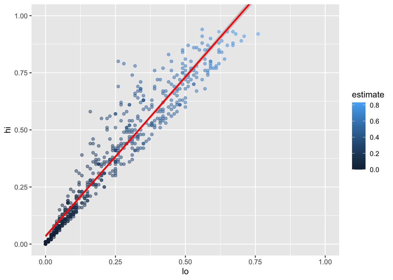
3.10 Do I need more practice with the tidyverse?
Absolutely: open a fresh file and begin by loading the tidyverse and the here package used to construct paths:
Next,
use here::here to construct a path to a file and readr::read_csv to read that file:
Parsed with column specification:
cols(
  person_id = col_character(),
  personal_name = col_character(),
  family_name = col_character()
)
We don’t need to write out fully-qualified names—here and read_csv will do—but
we will use them to make it easier to see what comes from where.
Next,
have a look at the tibble person,
which contains some basic information about a group of foolhardy scientists
who ventured into the Antarctic in the 1920s and 1930s in search of things best left undisturbed:
# A tibble: 5 x 3
  person_id personal_name family_name
  <chr>     <chr>         <chr>
1 dyer      William       Dyer
2 pb        Frank         Pabodie
3 lake      Anderson      Lake
4 roe       Valentina     Roerich
5 danforth  Frank         Danforth
How many rows and columns does this tibble contain?
[1] 5[1] 3(These names don’t have a package prefix because they are built in.)
Let’s show that information in a slightly nicer way
using glue to insert values into a string
and print to display the result:
person has 5 rows and 3 columnsIf we want to display several values,
we can use the function paste to combine the elements of a vector.
colnames gives us the names of a tibble’s columns,
and paste’s collapse argument tells the function
to use a single space to separate concatenated values:
person columns are person_id personal_name family_nameTime for some data manipulation. Let’s get everyone’s family and personal names:
# A tibble: 5 x 2
  family_name personal_name
  <chr>       <chr>
1 Dyer        William
2 Pabodie     Frank
3 Lake        Anderson
4 Roerich     Valentina
5 Danforth    Frank
and then filter that list to keep only those that come in the first half of the alphabet:
# A tibble: 3 x 2
  family_name personal_name
  <chr>       <chr>
1 Dyer        William
2 Lake        Anderson
3 Danforth    Frank
It would be more consistent to rewrite this as:
# A tibble: 3 x 2
  family_name personal_name
  <chr>       <chr>
1 Dyer        William
2 Lake        Anderson
3 Danforth    Frank
It’s easy to add a column that records the lengths of family names:
# A tibble: 5 x 4
person_id personal_name family_name name_length
<chr> <chr> <chr> <int>
1 dyer William Dyer 4
2 pb Frank Pabodie 7
3 lake Anderson Lake 4
4 roe Valentina Roerich 7
5 danforth Frank Danforth 8and then arrange in descending order:
person %>%
dplyr::mutate(name_length = stringr::str_length(family_name)) %>%
dplyr::arrange(dplyr::desc(name_length))# A tibble: 5 x 4
person_id personal_name family_name name_length
<chr> <chr> <chr> <int>
1 danforth Frank Danforth 8
2 pb Frank Pabodie 7
3 roe Valentina Roerich 7
4 dyer William Dyer 4
5 lake Anderson Lake 43.11 Key Points
install.packages('name')installs packages.library(name)(without quoting the name) loads a package.library(tidyverse)loads the entire collection of tidyverse libraries at once.read_csv(filename)reads CSV files that use the string ‘NA’ to represent missing values.read_csvinfers each column’s data types based on the first thousand values it reads.- A tibble is the tidyverse’s version of a data frame, which represents tabular data.
head(tibble)andtail(tibble)inspect the first and last few rows of a tibble.summary(tibble)displays a summary of a tibble’s structure and values.tibble$columnselects a column from a tibble, returning a vector as a result.tibble['column']selects a column from a tibble, returning a tibble as a result.tibble[,c]selects columncfrom a tibble, returning a tibble as a result.tibble[r,]selects rowrfrom a tibble, returning a tibble as a result.- Use ranges and logical vectors as indices to select multiple rows/columns or specific rows/columns from a tibble.
tibble[[c]]selects columncfrom a tibble, returning a vector as a result.min(...),mean(...),max(...), andstd(...)calculates the minimum, mean, maximum, and standard deviation of data.- These aggregate functions include
NAs in their calculations, and so will produceNAif the input data contains any. - Use
func(data, na.rm = TRUE)to removeNAs from data before calculations are done (but make sure this is statistically justified). filter(tibble, condition)selects rows from a tibble that pass a logical test on their values.arrange(tibble, column)orarrange(desc(column))arrange rows according to values in a column (the latter in descending order).select(tibble, column, column, ...)selects columns from a tibble.select(tibble, -column)selects out a column from a tibble.mutate(tibble, name = expression, name = expression, ...)adds new columns to a tibble using values from existing columns.group_by(tibble, column, column, ...)groups rows that have the same values in the specified columns.summarize(tibble, name = expression, name = expression)aggregates tibble values (by groups if the rows have been grouped).tibble %>% function(arguments)performs the same operation asfunction(tibble, arguments).- Use
%>%to create pipelines in which the left side of each%>%becomes the first argument of the next stage.
References
Wilkinson, Leland. 2005. The Grammar of Graphics. Springer.