The Cowichan Problems
Back in the 1990s, as the first wave of euphoria about parallel computing was topping out, I had a crazy idea: why don’t we actually try to measure, or at least compare, the usability of different parallel programming systems? I left the field before taking the idea very far, but with talk about clouds and GPUs growing louder by the day, I think the idea is worth revisiting; the proposal that Bruce Irvin and I put together is below the cut, and I’d be interested in feedback.
Most programmers believe that parallel programming is harder than sequential programming. We are developing a suite of simple problems that can be used to assess the usability of different scientific programming languages (parallel or otherwise) that captures modularization and integration concerns usually ignored by performance-oriented benchmark suites. This paper motivates and describes the suite.
Introduction
In the late 1980s and early 1990s, many people (including the first author of this paper) were convinced that programming was about to “go parallel” in a big way. Those same predictions are being made again today: fans of GPUs, multicore CPUs, and cloud computing all claim that programmers can no longer afford to not think about parallelism, and that we will have to rethink programming from the ground up to take advantage of all that shiny new hardware.
But how? And how will we know if we’re on the right track? Twenty years ago, a survey by Bal et al. listed more than 300 parallel programming systems [Bal 1989]. Only a handful have survived, all of them very conservative extensions to, or libraries for, mainstream languages. If Erlang, Haskell, ML, F#, or other exotic languages are to gain ground, their advocates must convince a sceptical audience that they actually can solve real problems more easily than existing alternatives.
We propose using a suite of simple problems to compare the usability of parallel programming systems. Competent programmers, fluent in a specific system, will implement solutions to these problems and report their experiences in terms of development time, code clarity, and runtime performance. These problems are individually very simple, but together cover a broad range of scientific domains.
One significant innovation in this work is that we also require implementors to chain applications together, so that the output of one is an input to another. This will allow us to assess how well each language or library supports modularization and re-use. It is also more realistic than having each application run in isolation, since large scientific codes are usually composed of modules that have different “best” data layouts and parallelization strategies.
History and Acknowledgments
The first author originally developed this suite in the mid-1990s, inspired by discussions with R. Bruce Irvin (then at the University of Wisconsin) and Henri Bal (Vrije Universiteit, Amsterdam), and by the work of Feo and others on the Salishan Problems [Feo 1992]. In recognition of the latter, this suite is called the Cowichan Problems (pronounced COW-i-chun); like Salishan, the word is a Northwest Coast native place name. Early experiences were described in [Wilson 1994] and [Bal 1996]. In 2009, Andrew Borzenko and Cameron Gorrie (then in the Department of Computer Science at the University of Toronto) re-wrote the earlier C implementation in C++ using several modern parallel programming systems.
Quantifying the Importance of Usability
Amdahl’s Law states that if tp is an algorithm’s running time on p processors and σ is the algorithm’s serial fraction (i.e., the fraction of the algorithm that cannot be parallelized), then:
| tp | = | σt1 + (1 – σ)t1/p |
The speedup on p processors is therefore:
| s(p) | = | t1/tp |
| = | t1/(σt1 + (1 – σ)t1/p) | |
| = | 1/(σ + (1 – σ)/p) |
As p→∞, the speedup is bounded by 1/σ. This makes intuitive sense: if 10% of an algorithm can’t be parallelized, then even with infinite hardware, the program can only be made to run 10 times faster.
But software doesn’t just happen: it has to be written and debugged, and these activities usually aren’t made faster by parallel hardware. (In fact, most programmers believe that doing parallel programming is harder and slower than doing it sequentially.) If we let T and S be the equivalents of t and s over the program’s whole lifetime, and D be its total development time, then:
| Tp | = | σT1 + (1 – σ)T1/p + D |
The achievable lifetime speedup is then:
| S∞ | = | 1/(σ + D/t1) |
The ratio of development time to run time therefore effectively increases the program’s serial fraction. Unless parallelization time can be substantially reduced, parallel programming will only be cost-effective when:
- the application is trivially parallel (e.g., task-farming a rendering calculation);
- the expected total program runtime is very large (i.e., the program is a package used extensively in a field such as computational chemistry or vehicle crash simulation); or
- cost is not an obstacle (i.e., the customer is Disney or the NSA).
The aim of this problem suite is to capture enough information about D to allow competing parallel programming systems to be ranked and compared.
Previous Work
Two comparative efforts in parallel programming are [Babb 1988] and [Feo 1992]. The first presented implementations of a simple numerical quadrature program in more than a dozen different parallel languages used on mid-1980s hardware. The second presented implementations of the Salishan Problems–Hamming number generation, isomer enumeration, skyline matrix reduction, and a simple discrete event simulator–in C*, Occam, Ada, and several dataflow and functional languages. Both books conveyed the flavor of the languages they describe, but neither compared languages or problem implementations directly.
More recently, Lutz has explored quantitative comparison of the relative productivity of different programming languages [Prechelt 2000, Prechelt 2009]. Our aim is to support replication of his work for parallel programming.
Methodology
Our aim is to assess and compare the usability of parallel programming systems. Here, we discuss issues related to choosing the problems that make up our benchmark suite, how to assess particular implementations, and other purposes which implementations of these might serve. Recognizing that our problems are extremely simple, we refer to them as “toys”.
Criteria for Selection
Our criteria for including toys are:
- Each toy should require no more than an hour to write and test in a well-supported sequential language. We feel that making individual problems more complicated will only discourage uptake.
- Correctness must be easy to verify. Toys whose output is easily visualized are therefore preferred, as are toys whose results are insensitive to floating-point effects.
- Speedup must similarly be easy to measure–while machine performance is not our focus, we are generally uninterested in parallel implementations that are slower than the sequential originals.
- At least some toys should not be “infinitely scalable”. Many real-world applications are not, and this suite should reflect such limitations.
- At least some toys should require I/O, since this important aspect of real-world programming is often neglected by PPS designers.
- There should be some overlap in the toys’ implementations, so that implementors can demonstrate how well their chosen systems take advantage of opportunities for code re-use.
- Together, the toys in the suite must exercise the parallel clichés discussed in the appendices. In particular,
- Toys should be specified by inputs and outputs rather than algorithmically, i.e., “sort N integers” rather than “parallelize quicksort”, so that implementors can choose algorithms that are “natural” for their systems. Implementations that parallelize a grossly inefficient sequential algorithm should be criticized for doing so.
Software Engineering Issues
The “single algorithm per program” model of many benchmarks is not representative of real programs, which often contain several qualitatively different phases or modules. A full implementation of this suite will therefore have two parts. In the first, each toy will be implemented as a stand-alone program. In the second, toys will be chained together as shown below. This will test the ease with which heterogeneous parallelism can be mixed within a single program. It will also show how well the system supports code re-use and information hiding, which are crucial to the development of large programs.
Where possible, chaining should execute toys concurrently. Some parallel programming systems impose extraneous constraints on programs, e.g., require all processes to participate in every barrier synchronization, or require the same executable to be loaded onto each processor. These constraints can limit the exploitation of potential concurrency. Permitting, but not requiring, concurrent execution of several toys should uncover such limitations.
Sizing
One crucial aspect of the specification of toys is the way in which the sizes of problems are determined. In a frozen model, the actual size of each problem and/or the number of processors available is compiled into each toy. A fully fluid implementation, by contrast, allows these sizes to be specified at run-time. If a system does not support fully-fluid implementations, it must at least use an intermediate model (which might be called slushy), in which the maximum size of individual problems is specified during compilation, but the actual size of a problem is only determined when the toy begins to execute.
Assessing Usability
One way to compare the usability of parallel programming systems would be to measure the performance achieved by an “average” programmer as a function of time on each toy. By analogy with Hockney’s n1/2 measure [Hockney 1991], we could in principle find the value of p1/2, i.e., the programming time required to achieve half of a machine’s peak performance for a particular combination of programming system and problem type. (Note that if performance was measured as a fraction of the figures quoted by manufacturers for their machines, it is unlikely that the halfway mark would ever be reached.) However, the number of implementors required is much greater than the number we can reasonably expect.
Alternatively, we could use code metrics to compare implementations of various toys. This is also dubious, both because [El Emam 2001] has shown that most metrics do little more than measure lines of code, and because of the difficulty of comparing metric values between languages.
The best we can hope for now is therefore qualitative consensus, e.g., to interview implementors about their experiences and ask other programmers who are familiar with the base languages used to read and comment on the parallel versions of the toys. We will also compare the length of code in parallel and sequential implementations, though we realize that this can exaggerate the impact of parallelization.
Other Uses for Implementations
This suite is intended for assessing the usability of parallel programming systems, but we envisage other uses. First, this suite will indicate what a mature parallel programming system should be able to support. In particular, we will ask implementors to describe how they debugged correctness and performance problems, and in particular what tools they used. (The lack of useful debugging tools is a chronic complaint among parallel programmers.)
This suite should also be useful for education, since toys will be small enough to be understood quickly, and parallelizing them should be a suitable classroom exercise in a senior undergraduate course on parallel computing.
The Problems
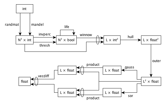
The chained implementation of these toys executes in the order shown below. Because of choices in steps 1 and 3, there are four possible chained sequences.
- An integer matrix
Iwithrrows andccolumns is created either by using the Mandelbrot Set algorithm (mandel) or by filling locations with random values (randmat). - The integer matrix
Iis shuffled in both dimensions (shuffle). - Either invasion percolation (
invperc) or histogram thresholding (thresh) is used to generate a Boolean maskBfromIin which the (minimum) percentage ofTruelocations isP. LikeI,Bhasrrows andccolumns. - The Game of Life (
life) is simulated forGgenerations, usingBas an initial configuration. This step overwrites the Boolean matrixB. - A vector of
L(m,x,y)points is created using the integer matrixIand the Boolean matrixB. - A series of convex hulls (
hull) are obtained from the points produced above. - The coordinates of the points from the previous step are normalized (
norm). - An
L×LmatrixAand anL-vectorVare created using the normalized point locations from the previous step (outer).`` - The matrix equation
AX=Vis solved using Gaussian elimination (gauss) and successive over-relaxation (sor) to generate two solution vectorsX<sub>gauss</sub>andX<sub>sor</sub>. These two toys should execute concurrently if possible. - The checking vectors
V<sub>gauss</sub>=AX<sub>gauss</sub>andV<sub>sor</sub>=AX<sub>sor</sub>are calculated (product). These two toys should execute concurrently if possible. - The norm-1 distance between
V<sub>gauss</sub>andV<sub>sor</sub>is calculated (vecdiff). This measures the agreement between the solutions found by the two methods.
The toys comprising the Cowichan Problems are sketched below.
gauss: Gaussian Elimination
This module solves a matrix equation AX=V for a dense, symmetric, diagonally dominant matrix A and an arbitrary vector non-zero V using explicit reduction. Input matrices are required to be symmetric and diagonally dominant in order to guarantee that there is a well-formed solution to the equation.
Inputs
matrix: the real matrix A.target: the real vector V.
Outputs
solution: a real vector containing the solution X.
hull: Convex Hull
Given a set of (x,y) points, this toy finds those that lie on the convex hull, removes them, then finds the convex hull of the remainder. This process continues until no points are left. The output is a list of points in the order in which they were removed, i.e., the first section of the list is the points from the outermost convex hull, the second section is the points that lay on the next hull, and so on.
Inputs
original: the vector of input points.
Outputs
ordered: the vector of output points (a permutation of the input).
invperc: Invasion Percolation
Invasion percolation models the displacement of one fluid (such as oil) by another (such as water) in fractured rock. In two dimensions, this can be simulated by generating an N×N grid of random numbers in the range [1..R], and then marking the center cell of the grid as filled. In each iteration, one examines the four orthogonal neighbors of all filled cells, chooses the one with the lowest value (i.e., the one with the least resistance to filling), and fills it in.
Filling begins at the central cell of the matrix (rounding down for even-sized axes). The simulation continues until some fixed percentage of cells have been filled, or until some other condition (such as the presence of trapped regions) is achieved. The fractal structure of the filled and unfilled regions is then examined to determine how much oil could be recovered.
The naïve way to implement this is to repeatedly scan the array. A much faster technique is to maintain a priority queue of unfilled cells which are neighbors of filled cells. This latter technique is similar to the list-based methods used in some cellular automaton programs, and is very difficult to parallelize effectively.
Inputs
matrix: an integer matrix.nfill: the number of points to fill.
Outputs
mask: a Boolean matrix filled withTrue(showing a filled cell) orFalse(showing an unfilled cell).
life: Game of Life
This module simulates the evolution of Conway’s Game of Life, a two-dimensional cellular automaton. At each time step, this module must count the number of live (True) cells in the 8-neighborhood of each cell using circular boundary conditions. If a cell has 3 live neighbors, or has 2 live neighbors and is already alive, it is alive in the next generation. In any other situation, the cell becomes, or stays, dead.
Inputs
matrix: a Boolean matrix representing the Life world.numgen: the number of generations to simulate.
Outputs
matrix: a Boolean matrix representing the world after simulation.
mandel: Mandelbrot Set Generation
This module generates the Mandelbrot Set for a specified region of the complex plane. Given initial coordinates (x0, y0), the Mandelbrot Set is generated by iterating the equation:
| x' | = | x2 – y2 + y0 |
| y' | = | 2xy + x0 |
until either an iteration limit is reached, or the values diverge. The iteration limit used in this module is 150 steps; divergence occurs when x2 + y2 becomes 2.0 or greater. The integer value of each element of the matrix is the number of iterations done. The values produced should depend only on the size of the matrix and the seed, not on the number of processors or threads used.
Inputs
nrows, ncols: the number of rows and columns in the output matrix.x0, y0: the real coordinates of the lower-left corner of the region to be generated.dx, dy: the extent of the region to be generated.
Outputs
matrix: an integer matrix containing the iteration count at each point in the region.
norm: Point Location Normalization
This module normalizes point coordinates so that all points lie within the unit square [0..1]×[0..1]. If xmin and xmax are the minimum and maximum x coordinate values in the input vector, then the normalization equation is
| xi' | = | (xi – xmin)/(xmax – xmin) |
y coordinates are normalized in the same fashion.
Inputs
points: a vector of point locations.
Outputs
points: a vector of normalized point locations.
outer: Outer Product
This module turns a vector containing point positions into a dense, symmetric, diagonally dominant N×N matrix by calculating the distances between each pair of points. It also constructs a real vector whose values are the distance of each point from the origin. Each matrix element Mi,j such that i ≠ j is given the value di,j, the Euclidean distance between point i and point j. The diagonal values Mi,i are then set to N times the maximum off-diagonal value to ensure that the matrix is diagonally dominant. The value of the vector element vi is set to the distance of point i from the origin, which is given by √(xi2 + yi2).
Inputs
points: a vector of (x,y) points, where x and y are the point’s position.
Outputs
matrix: a real matrix, whose values are filled with inter-point distances.vector: a real vector, whose values are filled with origin-to-point distances.
product: Matrix-Vector Product
Given a matrix A, a vector V, and an assumed solution X to the equation AX=V, this module calculates the actual product AX=V’, and then finds the magnitude of the error.
Inputs
matrix: the real matrix A.actual: the real vector V.candidate: the real vector X.
Outputs
e: the largest absolute value in the element-wise difference of V and V’.
randmat: Random Number Generation
This module fills a matrix with pseudo-random integers. The values produced must depend only on the size of the matrix and the seed, not on the number of processors or threads used.
Inputs
nrows, ncols: the number of rows and columns in the output matrix.s: the random number generation seed.
Outputs
matrix: an integer matrix filled with random values.
shuffle: Two-Dimensional Shuffle
This module divides the values in a rectangular two-dimensional integer matrix into two halves along one axis, shuffles them, and then repeats this operation along the other axis. Values in odd-numbered locations are collected at the low end of each row or column, while values in even-numbered locations are moved to the high end. An example transformation is:
| a | b | c | d | a | c | b | d | |
| e | f | g | h | → | i | k | j | l |
| i | j | k | l | e | g | f | h |
Note that how an array element is moved depends only on whether its location index is odd or even, not on whether its value is odd or even.
Inputs
matrix: an integer matrix.
Outputs
matrix: an integer matrix containing shuffled values.
sor: Successive Over-Relaxation
This module solves a matrix equation AX=V for a dense, symmetric, diagonally dominant matrix A and an arbitrary vector non-zero V using successive over-relaxation.
Inputs
matrix: the square real matrix A.target: the real vector V.tolerance: the solution tolerance, e.g., 10-6.
Outputs
solution: a real vector containing the solution X.
thresh: Histogram Thresholding
This module performs histogram thresholding on an image. Given an integer image I and a target percentage p, it constructs a binary image B such that Bi,j is set if no more than p percent of the pixels in I are brighter than Ii,j. The general idea is that an image’s histogram should have two peaks, one centered around the average foreground intensity, and one centered around the average background intensity. This program attempts to set a threshold between the two peaks in the histogram and select the pixels above the threshold.
Inputs
matrix: the integer matrix to be thresholded.percent: the minimum percentage of cells to retain.
Outputs
mask: a Boolean matrix whose values areTruewhere the value of a cell in the input image is above the threshold, andFalseotherwise.
vecdiff: Vector Difference
This module finds the maximum absolute elementwise difference between two vectors of real numbers.
Inputs
left: the first vector.right: the second vector.
Outputs
maxdiff: the largest absolute difference between any two corresponding vector elements.
winnow: Weighted Point Selection
This module converts a matrix of integers to a vector of points represented as x and y coordinates. Each location where mask is True becomes a candidate point, with a weight equal to the integer value in matrix at that location and x and y coordinates equal to its row and column indices. These candidate points are then sorted into increasing order by weight, and N evenly-spaced points selected to create the result vector.
Inputs
matrix: an integer matrix whose values are used as weights.mask: a Boolean matrix of the same size showing which points are eligible for consideration.nelts: the number of points to select.
Outputs
points: an N-vector of (x,y) points.
Other Issues
Input and Output
I/O is an important part of programming, but is often treated as being of secondary importance by language designers. This suite requires all stand-alone toys to read input values from files, and write results back; the chained version must be able to checkpoint intermediate results between toys. Finally, implementors are strongly encouraged to include some means of visualizing the output or evolution of individual toys.
The file formats used in the Cowichan Problems are specified in an appendix. Files are required to be human-readable (i.e., to use ASCII text). Implementations may also include I/O using binary (non-ASCII) files in whatever file formats are convenient. This will allow programmers to demonstrate the “natural” I/O capabilities of particular systems which most probably be used for checkpointing intermediate results in real programs.
Reproducibility
Reproducibility is an important issue for parallel programming systems. While constraining the order of operations in a parallel system to guarantee reproducibility makes programs in that system easier to debug, it can also reduce the expressiveness or performance of the system.
In this problem set, irreproducibility can appear in two forms: numerical and algorithmic. The first arises in toys such as gauss and sor, which use floating-point numbers. Precisely how round-off errors occur in these calculations can depend on the distribution of work among processors, or the order in which those processors carry out particular operations.
Irreproducibility also arises in toys which only use exact numbers, such as invperc and randmat. In the former, the percolation region is grown by repeatedly filling the lowest-valued cell on its perimeter. If several cells have this value, implementations may choose one arbitrarily. Thus, different implementations may produce very different fractal shapes. In the case of random number generation, the simplest thing to do is to run the same generator independently on each processor, although the values in the resulting matrix then depend on the number of processors used.
Bibliography
[Babb 1988] Robert G. Babb: Programming Parallel Processors. Addison-Wesley, 1988.
[Bal 1989]: Henri E. Bal, J. G. Steiner, and A. S. Tanenbaum: “Programming Languages for Distributed Computing Systems”. ACM Computing Surveys, 21(3), 1989.
[Bal 1996] Henri E. Bal and Gregory V. Wilson: “Using the Cowichan Problems to Assess the Usability of Orca”. IEEE Parallel & Distributed Technology, 4(3), 1996.
[Bennett 1990] John K. Bennett, John B. Carter, and Willy Zwaenepoel: “Munin: Distributed Shared Memory Based on Type-Specific Memory Coherence”. Proc. 1990 Conference on Principles and Practice of Parallel Programming, 1990.
[El Emam 2001] Khaled El Emam, Saida Benlarbi, Nishith Goel, and Shesh N. Rai: “The Confounding Effect of Class Size on the Validity of Object-Oriented Metrics”. IEEE Transasctions on Software Engineering, 27(7), 2001.
[Feo 1992] John T. Feo: A Comparative Study of Parallel Programming Languages: The Salishan Problems. North-Holland, 1992.
[Hockney 1991] Roger Hockney: “Performance Parameters and Benchmarking of Supercomputers”. Parallel Computing, 17, 1991.
[Prechelt 2000] Lutz Prechelt: “An Empirical Comparison of Seven Programming Languages”. IEEE Computer, 33(10), 2000.
[Prechelt 2000] Lutz Prechelt: “Plat_Forms: A Web Development Platform Comparison by an Exploratory Experiment Searching for Emergent Platform Properties”. IEEE Trans. Software Engineering, 2009.
[Wilson 1994] Gregory V. Wilson: “Assessing the Usability of Parallel Programming Systems: The Cowichan Problems”. Proc. IFIP Working Conference on Programming Environments for Massively Parallel Distributed Systems, Birkhäuser, 1994.
File Formats
Vector
A vector file begins with a single positive integer, which specifies the number of elements in the vector. This is then followed by N rows, each containing a single value.
Matrix
A file containing a matrix begins with a pair of positive integers, which specify the number of rows and columns in the matrix respectively. (Note that this means the first number is the Y extent, and the second number is the X extent.) Elements of the vector or matrix then appear one per line in order of increasing index, i.e., the element at (1,1) appears first, then the element at (1,2), and so on up to (1,N), which is followed by the element at index (2,1).
Basic Types
Vectors and matrices may contain Booleans, integers, or reals; vectors may also contain (x,y) points. The two Boolean values are represented by upper-case ‘T’ and ‘F’. Integers and reals are represented in the usual way; points are represented as two numbers separated by a single space character.
Parallel Operations
This list details some operations which are supported by many parallel programming systems. The toys described above provide opportunities for exercising many of these, and implementors are encouraged to phrase discussion of their work in terms of these operations where appropriate.
- elementwise operations on arrays (unary, binary, and scalar promotion)
- cumulative operations on arrays (reduction and parallel prefix)
- array re-shaping and re-sizing (e.g., sub-array extraction)
- partial (conditionally masked) versions of all of the above
- regular data motion (e.g., circular and planar shifting)
- irregular data motion (e.g., 1-to-1, 1-to-many, and many-to-1 permutation)
- scalar and non-scalar value location (e.g., finding a scalar or record value in an array)
- differential local addressing (i.e., subscripting an array with an array)
- full or partial replication of shared read-only values
- full or partial replication of shared read-mostly values with automatic consistency management
- structures with rotating ownership, suitable for migration
- producer-consumer structures
- partitionable structures
- pre-determined run-time re-partitioning (i.e., re-distributing an array)
- dynamic re-partitioning (e.g., for load balancing)
- committed mutual exclusion (e.g., waiting on a semaphore)
- uncommitted mutual exclusion (e.g., lock or fail)
- barrier synchronization
- multiple concurrent barriers used by non-overlapping groups of processes
- fetch-and-add, and other fetch-and-operate functions
- pre-scheduled receipt of messages of known composition
- variable-length message receipt
- message selection by type
- message selection by source
- message selection by contents
- guarded message selection (e.g., CSP’s
altconstruct) - broadcast and partial broadcast
- split-phase (non-blocking) operations
- data marshalling and unmarshalling of “flat” structures (e.g., arrays of scalars)
- data marshalling and unmarshalling of nested or linked structures
- heterogeneous parallelism (i.e., running different applications concurrently in one machine)
- pipelining
- distributed linked structures in systems without physically-shared memory
- indexing of distributed shared arrays
- collective I/O
- uniform-size interleaved I/O
- heterogeneous-size interleaved I/O
- independent I/O operations on a single shared file
Memory Reference Patterns
These are inspired by the categorization originally used in the Munin system [Bennett 1990]. Again, implementors are encouraged to phrase discussion of their work in these terms where appropriate.
- Write-once: variables which are assigned a value once, and only read thereafter. These can be supported through replication.
- Write-many: variables which are written and read many times. If several processes write to the variable concurrently, they typically write to different portions of it.
- Producer-consumer: variables which are written to by one or more objects, and read by one or more other objects. Entries in a shared queue, or a mailbox used for communication between two processes, are examples.
- Private: variables which are potentially shared, but actually private. The interior points of a mesh in a program which uses geometric decomposition fall into this category, while boundary points belong to the previous class.
- Migratory: variables which are read and written many times in succession by a single process before ownership passes to another process. The structures representing particles in an N-body simulation are the clearest example of this category.
- Result: Accumulators which are updated many times by different processes, but thereafter read.
- Read-mostly: Any variable which is read much more often than it is written to. The best score so far in a search problem is a typical instance of this class: while any process might update it, in practice processes read its value much more often than they change it.
- Synchronization: Variables used to force explicit synchronization in a program, such as semaphores and locks. These are typically ignored for long periods, and then the subject of intense bursts of access activity.
- General read-write: Any variable which cannot be put in one of the above categories.